

HGCN论文模型代码follow
1、摘要
- 论文解决的问题是什么?
In this paper, we study the problem
of heterogeneous graph-enhanced relational learning for recom-
mendation.
在推荐系统里面解决异构图增强学习
- 框架的理解:
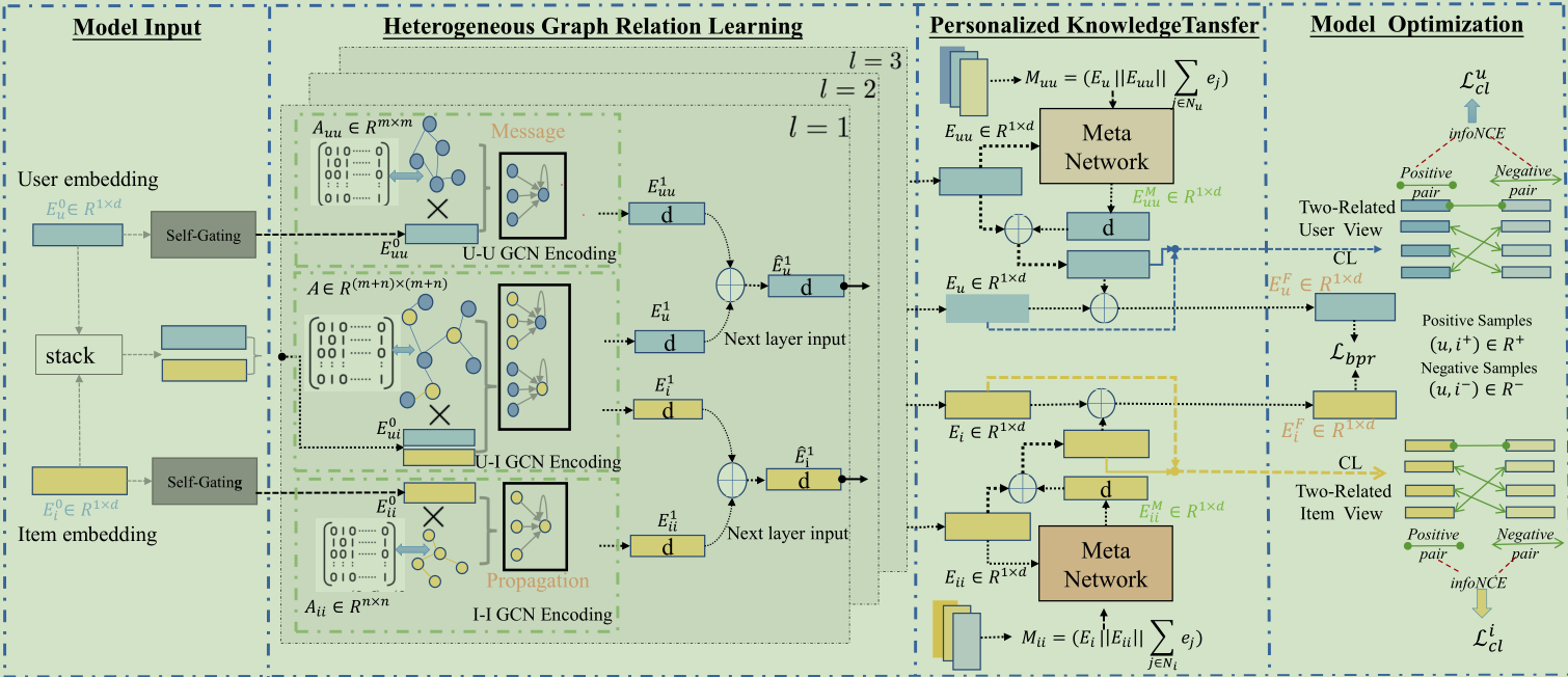
Heterogeneous Graph Contrastive Learning (HGCL):异构图对比学习
①这个框架可以能够将异构关系语义合并到结合到用户-项目交互建模中
②鉴于异构边信息heterogeneous side information在用户和物品不同,使用元网络meta networks增强异构图对比学习,以允许具有自适应对比增强的个性化知识转换器
- 实验效果:
The experimental results on three real-world datasets
demonstrate the superiority of HGCL over state-of-the-art recom-
mendation methods. Through ablation study, key components in
HGCL method are validated to benefit the recommendation perfor-
mance improvement. The source code of the model implementation
is available at the link https://github.com/HKUDS/HGCL.
在三个数据集上进行了研究,比最先进的state-of-the-art推荐系统的方法好。
并且进行了消融实验。消融实验的理解:
:::primary
消融研究对于深度学习研究至关重要。理解系统中的因果关系是产生可靠知识的最直接方式(任何研究的目标)。消融是一种非常省力的方式来研究因果关系。
如果您采用任何复杂的深度学习实验设置,您可能会删除一些模块(或用随机的模块替换一些训练有素的功能)而不会降低性能。消除研究过程中的噪音:进行消融研究。
如果您无法完全理解您的系统?很多活动部件,想确定它的工作原因是否与您的假设密切相关?尝试删除东西。花费至少约10%的实验时间来诚实地反驳你的论文。
:::
2、介绍(INTRODUCTION)
①GNN在推荐系统里面编码用户和商品的关系中大放异彩,关键思想是通过聚合图传播层上的邻居的特征信息来学习节点表示(节点包括user和item)。但是现在很多基于GNN的协同过滤模型collaborative filtering (CF) models仅关注同质信息。HGCL解决了这个问题。
②当前大部分的异构图神经网络受到了稀疏训练标签的限制,即目前的异构图神经网络对标签很敏感,可能会因此没法产生高质量的user/item embeddings,用于模型优化。所以引入了图对比自监督学习Contrastive self-supervised learning,GCL可以有效解决缺乏足够观察标签的问题。GCL的核心思想:正对比样本的表示之间的一致性将被最大化,而负对的嵌入之间的距离将被推开(应该是最小化的意思?)。
③边信息之间的依赖关系和用户-物品交互建模往往不是单一的,而是具有多样性的。本文学习了一个对比增强器contrastive augmentor
本文实质上要解决的问题:
- 如何有效地跨不同视图迁移辅助知识
- 如何通过个性化增强进行异构关系对比学习
进入框架:
- 利用
异质图神经网络作为编码器,在编码嵌入中保留了异质关系的丰富语义。 - 为了应对个性化增强,我们提出了一个定制的对比学习框架,该框架设计了一个
元网络来编码用户和项目的个性化特征。它允许我们执行特定于用户和项目的增强,以跨不同的关系视图传递信息信号。
怎么感觉这篇论文像把别人的工作缝合起来就变成了自己的工作捏
3、相关的工作
3.1 基于gnn的推荐系统
3.2 推荐系统中的对比学习
对比自监督学习生成的自监督信号可以用来丰富用户表示学习。在推荐系统中,对比学习可以成为一个强大的工具,将自监督信号与对比表示视图之间的对齐结合起来进行数据增强。
3.3 异构图学习
4、方法
ok,进入框架的具体部分咯
4.1 符号表示
- 用户-商品图:$\mathcal{G} _{ui}={\mathcal{V} _u,\mathcal{V} _i,\mathcal{E} _{ui}}$
$\mathcal{V} _u$:用户集合
$\mathcal{V} _i$:物品集合
$\mathcal{E}_{\mathcal{U}\boldsymbol{i}}$:边的集合,里面的边说明用户u和物品i有过互动
- 用户-用户图:$G_{uu}={\mathcal{V}{u},\mathcal{E}{uu}}$
$\mathcal{E}_{\mathcal{u}\boldsymbol{u}}$:里面的边说明两个用户有过互动
- 物品-物品图:$G_{ii}={\mathcal{V}{i},\mathcal{E}{ii}}$
$\mathcal{E}_{\mathcal{i}\boldsymbol{i}}$:里面的边说明两个物品在外部知识里面有联系(比如属于同一类物品)
三个邻接矩阵:$\mathbf{A}{ui}\in\mathbb{R}^{m\times n},\mathbf{A}{uu}\in\mathbb{R}^{m\times m},\mathbf{A}_{ii}\in\mathbb{R}^{n\times n}$。
这个图就要用来预测用户和物品之间未观察到的交互
4.2 异构图关系学习
4.2.1 关系感知embedding初始化
使用
xavier initializer对id-corresponding embeddings $\mathbf{e}_u,\mathbf{e}_i\in\mathbb{R}^d$进行初始化,d代表隐藏的维度,代码如下:# 初始化权重,hide_dim是隐藏层深度,为d
def init_weight(self, userNum, itemNum, hide_dim):
initializer = nn.init.xavier_uniform_
embedding_dict = nn.ParameterDict({
'user_emb': nn.Parameter(initializer(t.empty(userNum, hide_dim))),
'item_emb': nn.Parameter(initializer(t.empty(itemNum, hide_dim))),
})
return embedding_dict代码解读:
- 这段代码是一个类的方法,用于初始化权重。它接受三个参数:
userNum表示用户数量,itemNum表示物品数量,hide_dim表示隐藏层的维度(或深度)。 - 在方法内部,首先创建了一个
nn.ParameterDict对象来存储权重参数。nn.ParameterDict是PyTorch中的一种数据结构,用于保存一组参数。参数被定义为nn.Parameter对象,并使用指定的初始化器进行初始化。 - 在这里,使用了Xavier均匀分布初始化器
nn.init.xavier_uniform_,它会根据指定的形状生成均匀分布的随机数,并将其作为参数的初始值。 - 最后,方法返回了这个
embedding_dict对象,它将在模型的其他部分使用到初始化权重。
在主要模型里面,代码体现在:
# Initialize Embeddings
userembed0 = self.embedding_dict['user_emb'].weight
itemembed0 = self.embedding_dict['item_emb'].weight- 这段代码是一个类的方法,用于初始化权重。它接受三个参数:
特定于节点的embedding(
node-specific embeddings)形成了初始的embedding矩阵$\mathbf{E}_{\boldsymbol{u}}^0\in\mathbb{R}^{\boldsymbol{m}\times d}$和$\mathbf{E}_i^0\in\mathbb{R}^{\boldsymbol{n}\times\boldsymbol{d}}$,这两个初始的矩阵分别被送入了不同的图编码器, user-item域, user-user域,item-item域。为了突出这三种关系类型之间交互模式的差异,训练了一个自门控模块去派生出用户社会联系和物品语义联系的关系感知嵌入(
relation-aware embeddings),公式如下:$$\mathbf{E}{uu}^0=\mathbf{E}_u^0\odot\sigma(\mathbf{E}_u^0\mathbf{W}_g+\mathbf{b}_g);\quad\mathbf{E}{ii}^0=\mathbf{E}_i^0\odot\sigma(\mathbf{E}_i^0\mathbf{W}_g+\mathbf{b}_g)$$# 用户的relation-aware embeddings
def self_gatingu(self,em):
return torch.multiply(em, torch.sigmoid(torch.matmul(em,self.gating_weightu) + self.gating_weightub))
# 物品语义联系的relation-aware embeddings
def self_gatingi(self,em):
return torch.multiply(em, torch.sigmoid(torch.matmul(em,self.gating_weighti) + self.gating_weightib))其中$\mathbf{E}_\text{uu }^0\in\mathbb{R}^{m\times d}$代表同构图${\mathcal{G}}\text{uu}$的embedding,$\mathbf{E}{ii}^0\in\mathbb{R}^{\boldsymbol{n}\times d}$代表同构图${\mathcal{G}}_\text{ii}$的embedding。σ(i)代表
sigmoid激活函数,⊙ 表示逐元素乘法运算。通过这个乘法跳跃连接的自门机制,$\mathbf{E}_\text{uu }^0$,$\mathbf{E}_\text{ii}^0$不仅与初始的embedding共享共同语义,同时在表现user-user和item-item关系方面也更加灵活
在主要模型里面,代码内容体现在:
# 通过self_gatingu和self_gatingi对它们进行自门控处理,得到uu_embed0和ii_embed0 |
4.2.2 异质消息传播
- 首先应用图卷积神经网络作为图结构三视图的编码器。以用户-物品关系图为例详细阐述建模过程:
- 对于图$\mathcal{G} {ui}$, HGCL迭代细化用户和物品嵌入,如下:$\mathbf{e}u^{l+1}=\sum{i\in\mathcal{N}u}\frac1{\sqrt{|\mathcal{N}_u|}\sqrt{|\mathcal{N}_i|}}\mathbf{e}_i^l;\quad\mathbf{e}_i^{l+1}=\sum{u\in\mathcal{N}_i}\frac1{\sqrt{|\mathcal{N}_i|}\sqrt{|\mathcal{N}_u|}}\mathbf{e}_u^l$,其中$\mathcal{N}{\mathcal{u}}$和$\mathcal{N}_{\mathcal{i}}$代表目标节点u和i的邻居集合。$\mathbf{e}_u^l,\mathbf{e}_i^l\in\mathbb{R}^d$表示在第$l$轮循环中user u和item i的 embedding向量。
- $\mathbf{e}_u^0,\mathbf{e}_i^0$是embedding矩阵$\mathbf{E}_u^0,\mathbf{E}_i^0$的行向量。
- 关系感知消息传递范式没有进行转换和非线性激活。
对于GCN图神经网络的定义,如下面代码所示:
class GCN_layer(nn.Module): |
一、首先先来看这个sparse_mx_to_torch_sparse_tensor函数。
1、if type(sparse_mx) != sp.coo_matrix: sparse_mx = sparse_mx.tocoo().astype(np.float32).
这段代码首先判断判断输入的稀疏矩阵 sparse_mx 的类型是否为 scipy.sparse.coo_matrix,如果不是,则将其转换为 coo_matrix 类
2、indices = torch.from_numpy(np.vstack((sparse_mx.row, sparse_mx.col)).astype(np.int64))
这段代码的目的是创建一个稀疏矩阵中非零元素的索引张量 indices。
首先,sparse_mx.row 是稀疏矩阵 sparse_mx 中非零元素所在的行索引数组。sparse_mx.col 是稀疏矩阵 sparse_mx 中非零元素所在的列索引数组。
接下来,np.vstack((sparse_mx.row, sparse_mx.col)) 将行索引和列索引数组按垂直方向进行堆叠,形成一个形状为 (2, nnz) 的数组,其中 nnz 是稀疏矩阵中非零元素的数量。在堆叠后的数组中,第一行是非零元素的行索引,第二行是非零元素的列索引。
最后,torch.from_numpy 将上述数组转换为 PyTorch 张量 indices。这个张量存储了稀疏矩阵中非零元素的行索引和列索引,每一列对应一个非零元素的位置 (row_index, col_index)。
二、看看def normalize_adj(self, adj)这段代码
首先,代码使用 sp.coo_matrix(adj) 将输入的邻接矩阵 adj 转换为 scipy.sparse.coo_matrix 类型的稀疏矩阵。这是为了确保邻接矩阵的表示形式符合 COO 格式的要求。
接下来,代码计算每个节点的度数(degree)之和 rowsum,即邻接矩阵每一行的元素之和。这里使用 adj.sum(1) 对邻接矩阵的每一行进行求和操作,得到一个形状为 (n, 1) 的数组,其中 n 是节点的数量。
然后,代码计算每个节点度数的倒数的平方根 d_inv_sqrt,通过对 rowsum 进行 -0.5 次幂运算得到。注意,为避免除以 0 的情况,代码使用 np.isinf 函数将无穷大的元素置为 0。
然后,代码计算每个节点度数的倒数的平方根 d_inv_sqrt,通过对 rowsum 进行 -0.5 次幂运算得到。注意,为避免除以 0 的情况,代码使用 np.isinf 函数将无穷大的元素置为 0。
接着,代码构建对角矩阵 d_mat_inv_sqrt,其中对角线元素为 d_inv_sqrt,其余元素为 0。这里使用 sp.diags 函数创建对角矩阵。
最后,代码执行对称归一化操作,根据公式 D^(-0.5) * A * D^(-0.5),其中 D 是 d_mat_inv_sqrt 对角矩阵,A 是输入的邻接矩阵。这里使用矩阵乘法 dot 进行计算,并将结果转换为 COO 稀疏矩阵表示形式。
最终,函数返回对称归一化后的邻接矩阵,以 COO 稀疏矩阵的形式返回。
三、前向传递forward函数
这段代码是一个图神经网络的前向传播函数。它接受节点的特征矩阵 features,图的邻接矩阵 Mat,以及需要更新的节点索引 index。
subset_Mat = Mat:将输入的邻接矩阵Mat赋值给变量subset_Mat。subset_features = features:将输入的节点特征矩阵features赋值给变量subset_features。subset_Mat = self.normalize_adj(subset_Mat):调用self.normalize_adj函数对subset_Mat进行对称归一化操作,得到归一化后的邻接矩阵。subset_sparse_tensor = self.sparse_mx_to_torch_sparse_tensor(subset_Mat).cuda():将归一化后的邻接矩阵转换为稀疏张量,并将其移动到 GPU 上。self.sparse_mx_to_torch_sparse_tensor是一个辅助函数,将稀疏矩阵转换为 PyTorch 中的稀疏张量表示。out_features = torch.spmm(subset_sparse_tensor, subset_features):利用稀疏矩阵-稠密矩阵乘法(Sparse Matrix-Dense Matrix Multiplication,spmm)操作,将归一化后的邻接矩阵subset_sparse_tensor与节点特征矩阵subset_features相乘,得到输出特征out_features。new_features = torch.empty(features.shape).cuda():创建一个与输入特征矩阵features相同形状的空张量new_features,并将其移动到 GPU 上。new_features[index] = out_features:将输出特征out_features赋值给new_features的指定索引index,更新对应节点的特征。dif_index = np.setdiff1d(torch.arange(features.shape[0]), index):使用np.setdiff1d函数计算出不在索引index中的节点索引集合dif_index。new_features[dif_index] = features[dif_index]:将输入特征矩阵features中不在索引index中的节点特征复制到new_features中,保持这些节点的特征不变。return new_features:返回更新后的节点特征矩阵new_features。
在主要模型里面,代码体现在:
# 进入编码器的循环,对每个编码器层进行处理。 |
4.2.3 异构信息聚合
每次迭代中的信息都是从异质关系中聚合而来。
- 通过异构消息传播的多次迭代,高阶嵌入通过多跳连接保留异构语义。特别地,user和item的embdding以下定义的异构融合过程进行更新:
$$\widehat{\mathbf{E}}u^{l+1}=f(\mathbf{E}u^{l+1},\mathbf{E}{uu}^{l+1});\quad\widehat{\mathbf{E}}_i^{l+1}=f(\mathbf{E}_i^{l+1},\mathbf{E}{ii}^{l+1})$$
第$l$+1轮迭代中的embedding $\widehat{\mathbf{E}}_u^{l+1}\in\mathbb{R}^{m\times d},\widehat{\mathbf{E}_i}^{\boldsymbol{l}+1}\in\mathbb{R}^{\boldsymbol{n}\times d}$整合了异构语义,成为下一层的输入,$f$代表异构信息融合函数,出于降低模型复杂度的考虑,用逐元素均值池化作为融合函数$f(·)$
代码体现在:
# Aggregation of message features across the two related views in the middle layer then fed into the next layer |
为了用编码的特定层表示进一步聚合异质信息,生成user和item的整体embedding:$$\mathbf{E}u=\mathbf{E}u^0+\sum{l=1}^L\frac{\mathbf{E}_u^l}{||\mathbf{E}_u^l||};\quad\mathbf{E}_i=\mathbf{E}_i^0+\sum{l=1}^L\frac{\mathbf{E}_i^l}{||\mathbf{E}_i^l||}$$,其中$l$代表
GCN的最大迭代次数,每个GCN层的输出归一化。使用跳跃连接添加初始嵌入$\mathbf{E}_u^0,\mathbf{E}_i^0$,上述公式表明了用户-项目交互视图的特定层表示聚合。代码具体体现在:
self.userEmbedding = t.stack(self.all_user_embeddings, dim=1)
self.userEmbedding = t.mean(self.userEmbedding, dim = 1)
self.itemEmbedding = t.stack(self.all_item_embeddings, dim=1)
self.itemEmbedding = t.mean(self.itemEmbedding, dim = 1)
self.uiEmbedding   = t.stack(self.all_ui_embeddings, dim=1)
self.uiEmbedding   = t.mean(self.uiEmbedding, dim=1)
self.ui_userEmbedding, self.ui_itemEmbedding = t.split(self.uiEmbedding, [self.userNum, self.itemNum])
pytorch代码解释:
self.userEmbedding = t.stack(self.all_user_embeddings, dim=1):将self.all_user_embeddings中的嵌入向量按照维度1进行堆叠,得到一个新的张量self.userEmbedding。这里假设self.all_user_embeddings是一个包含多个嵌入向量的列表或张量,维度为(embedding_dim, num_user_embeddings)。self.userEmbedding = t.mean(self.userEmbedding, dim=1):对self.userEmbedding进行维度1上的平均池化操作,得到一个平均后的用户嵌入向量。这里假设self.userEmbedding是一个维度为(embedding_dim, num_user_embeddings)的张量,通过对维度1上的元素求平均,得到一个维度为(embedding_dim,)的用户嵌入向量。self.itemEmbedding = t.stack(self.all_item_embeddings, dim=1):类似于第一行的操作,将self.all_item_embeddings中的嵌入向量按照维度1进行堆叠,得到一个新的张量self.itemEmbedding。self.itemEmbedding = t.mean(self.itemEmbedding, dim=1):类似于第二行的操作,对self.itemEmbedding进行维度1上的平均池化操作,得到一个平均后的物品嵌入向量。self.uiEmbedding = t.stack(self.all_ui_embeddings, dim=1):类似于第一行的操作,将self.all_ui_embeddings中的嵌入向量按照维度1进行堆叠,得到一个新的张量self.uiEmbedding。self.uiEmbedding = t.mean(self.uiEmbedding, dim=1):类似于第二行的操作,对self.uiEmbedding进行维度1上的平均池化操作,得到一个平均后的用户-物品组合嵌入向量。self.ui_userEmbedding, self.ui_itemEmbedding = t.split(self.uiEmbedding, [self.userNum, self.itemNum]):将self.uiEmbedding按照给定的索引进行拆分,得到用户嵌入向量和物品嵌入向量。具体来说,self.uiEmbedding的形状应该为(embedding_dim, num_ui_embeddings),其中num_ui_embeddings是用户-物品组合的数量。然后,通过t.split函数将self.uiEmbedding按照索引[self.userNum, self.itemNum]进行拆分,得到两个张量self.ui_userEmbedding和self.ui_itemEmbedding,分别表示用户和物品的嵌入向量。
user-user和item-item的嵌入是以类似的方式通过多阶信息聚合得到的。
代码也在上面了。
4.3 跨视图元网络
4.3.1 元知识提取
提炼出的用户-用户关系视图和物品-物品关系视图的元知识如下:
$\mathbf{M}{\boldsymbol{u}\boldsymbol{u}}=\mathbf{E}{\boldsymbol{u}}||\mathbf{E}{\boldsymbol{u}\boldsymbol{u}}||\sum{\boldsymbol{i}\in\mathcal{N}{\boldsymbol{u}}}\mathbf{e}{i};\quad\mathbf{M}{\boldsymbol{i}\boldsymbol{i}}=\mathbf{E}{i}||\mathbf{E}{\boldsymbol{i}\boldsymbol{i}}||\sum{\boldsymbol{u}\in\mathcal{N}{\boldsymbol{i}}}\mathbf{e}{\boldsymbol{u}}$,其中$\mathbf{M}{uu}\in\mathbb{R}^{m\times3d},\mathbf{M}{ii}\in\mathbb{R}^{n\times3d}$表示编码上下文信息的元知识,分别为用户和项目侧知识生成个性化的知识迁移函数。
除此之外,将邻域信息纳入元知识中。
辅助域的embedding表征了用户的社会影响力和项目的语义相关性
具体代码展示如下:
# Meta-knowlege extraction |
代码解读:
tembedu = (self.meta_netu(t.cat((auxiembedu, targetembedu, uneighbor), dim=1).detach())):该行代码将辅助用户嵌入向量 (auxiembedu)、目标用户嵌入向量 (targetembedu) 和目标用户的邻居信息 (uneighbor) 连接起来,并将连接后的向量作为输入传递给名为self.meta_netu的元网络。self.meta_netu对输入进行处理,得到用户的元嵌入向量tembedu。detach()的作用是将输入的梯度信息断开,以避免在元网络的计算过程中对原始输入进行梯度传播。
4.3.2个性化跨视角知识迁移
- 在HGCL中,提取的元知识用于生成具有定制变换矩阵的参数化知识传输网络.所提出的元神经网络是:
$$\left{\begin{aligned}f_{mlp}^1(\mathbf{M}{uu})&\to\mathbf{W}{uu}^{M1}\f_{mlp}^2(\mathbf{M}{uu})&\to\mathbf{W}{uu}^{M2}\end{aligned}\right.$$
$f_{mlp}^1,f_{mlp}^1$是元知识学习器,由两个具有 PReLU 激活函数的全连接层组成。这些函数将元知识$M_{uu}$作为输入,输出自定义的transformation矩阵$\mathbf{W}{\boldsymbol{u}\boldsymbol{u}}^{\boldsymbol{M}1}\in\mathbb{R}^{\boldsymbol{m}\times d\times\boldsymbol{k}},\mathbf{W}{\boldsymbol{u}\boldsymbol{u}}^{\boldsymbol{M}2}\in\mathbb{R}^{\boldsymbol{m}\times\boldsymbol{k}\times\boldsymbol{d}}$。两个参数张量都包含 n 个矩阵,每个矩阵为 n 个用户。这两组矩阵将变换的秩限制为$k<d$.
一、先来看看MLP部分的代码:
class MLP(torch.nn.Module): |
先看forward函数。如果 feature_pre 为 True,则将输入数据 data 通过线性层 linear_pre 进行特征预处理。使用 PReLU(带参数的修正线性单元)激活函数对输入进行非线性变换。通过多个隐藏层进行数据的转换,每个隐藏层包含一个线性层和一个 tanh 激活函数。如果 dropout 为 True,在每个隐藏层后应用 dropout 操作,用于随机丢弃一部分神经元,以防止过拟合。通过线性层 linear_out 进行最终的输出,并对输出进行 L2 归一化操作。返回处理后的结果。
二、再来看一下具体提取出来的元神经网络部分的代码(以user部分的为例)
# Low rank matrix decomposition 低秩矩阵分解 |
利用生成的参数矩阵和非线性映射函数来构建我们的定制传输网络:
$\mathbf{E}{uu}^M=\sigma(\mathbf{W}{uu}^{M1}\mathbf{W}{uu}^{M2}\mathbf{E}{uu})$
其中,$\sigma(·)$代表
PReLU激活函数,$\mathbf{E}_\text{uu }^M\in\mathbb{R}^{m\times d}$包含通过自定义映射转换的嵌入用户-用户社交视图的函数ok,多说无益,再看一下具体的代码模块:
# The learned matrix as the weights of the transformed network
    tembedus = (t.sum(t.multiply( (auxiembedu).unsqueeze(-1), low_weightu1), dim=1))
    # Equal to a two-layer linear network;
    # Ciao and Yelp data sets are plus gelu activation function
    tembedus =  t.sum(t.multiply((tembedus)  .unsqueeze(-1), low_weightu2), dim=1)
    tembedis = (t.sum(t.multiply((auxiembedi).unsqueeze(-1), low_weighti1), dim=1))
    tembedis =  t.sum(t.multiply((tembedis)  .unsqueeze(-1), low_weighti2), dim=1)
    transfuEmbed = tembedus
    transfiEmbed = tembedis
然后利用定制的嵌入来增强从用户-项目交互中编码的用户嵌入。用户的融合过程通过以下加权求和进行:
$\mathbf{E}u^F=\alpha_u\mathbf{E}_u+(1-\alpha_u)(\mathbf{E}_{uu}+\mathbf{E}{uu}^M)$
其中$\alpha_{u}\in\mathbb{R}$表示控制用户-物品交互视图嵌入和用户-用户社交视图嵌入之间权重的超参数。在这里,用户-用户关系视图的原始嵌入也被用于更好的优化。$\mathbf{E}_{\boldsymbol{u}}^{F}\in\mathbb{R}^{\boldsymbol{m}\times d}$代表最终的embedding
4.4 用于增强的异质关系对比学习
4.4.1 跨视图对比学习
- 设计了跨视图对比学习范式来增强具有自增强的异构关系学习的鲁棒性。具体来说,两个辅助视图($\mathbf{E}{\boldsymbol{uu}}^{\boldsymbol{M}}$,$\mathbf{E}{ii}^{\boldsymbol{M}}$)的嵌入与用户-项目交互视图($E_u$和$E_i$)。在这种设计下,辅助视图的嵌入作为有效的正则化来影响具有自监督信号的用户-物品交互建模。
- 为了通过考虑个性化的跨视图知识迁移来捕捉多样化的用户偏好,我们将个性化的跨视图知识迁移与对比学习集成在我们的推荐系统中。特别的,跨视图嵌入对齐在不同的表示视图之间以自适应的方式进行。
- 辅助视图特定的嵌入$E_{uu},E_{ii}$通过元网络生成的个性化映射函数进行处理,以生成个性化的辅助嵌入$\mathbf{E}^M,\mathbf{E}{ii}^M$
4.4.2 基于InfoNCE的对比度损失
在异构图关系学习和跨视图元网络的帮助下,获得了用户和项目的两组embedding(用户:$\mathbf{E}{\boldsymbol{uu}}^{\boldsymbol{M}},\mathbf{E}{\boldsymbol{u}}$,物品:$\mathbf{E}_{ii}^M,\mathbf{E}_i$)
- 使用基于infonce的两种表示视图之间的对比学习损失来增强我们的HGCL方法的用户/项目表示学习,如下所示:
$\mathcal{L}{cl}^u=\sum{u\in\mathcal{V}u}-\log\frac{\exp\left(s(\mathbf{e}{uu}^M+\mathbf{e}{uu},\mathbf{e}{u})/\tau\right)}{\sum_{u^{\prime}\in\mathcal{V}u}\exp\left(s(\mathbf{e}{uu}^M+\mathbf{e}{uu},\mathbf{e}{u}^{\prime})/\tau\right)}$
其中$\mathbf{e}{\boldsymbol{uu}}^M\in\mathbb{R}^d,\mathbf{e}{\boldsymbol{u}}\in\mathbb{R}^d$分别是来自矩阵的嵌入向量$\mathbf{E}{uu}^M,\mathbf{E}{u}$. S(·) 表示相似度函数,可以是内积或余弦相似度,这里使用余弦相似度。τ代表温度系数,能够自动识别困难的负样本。
先来看一下相似度的代码函数展示:
def score(x1,x2): |
用于对输入的嵌入矩阵进行行和列的随机置换的代码:
def row_column_shuffle(embedding): |
完整的代码:
def metaregular(self,em0,em,adj): |
Adj_Norm = t.from_numpy(np.sum(adj, axis=1)).float().cuda()计算邻接矩阵adj每行的和,并转换为PyTorch张量,并将其转移到GPU上。adj = self.sparse_mx_to_torch_sparse_tensor(adj)将邻接矩阵adj转换为稀疏张量的表示形式。edge_embeddings = torch.spmm(adj.cuda(), user_embeddings) / Adj_Norm使用稀疏矩阵-向量乘法计算边的嵌入向量。首先,将邻接矩阵adj与用户嵌入矩阵user_embeddings相乘,然后除以Adj_Norm进行归一化。
相似的,可以获得物品方面的InfoNCE损失$\mathcal{L}_{\boldsymbol{c}\boldsymbol{l}}^i$
最后,总的对比损失$\mathcal{L}_{cl}=\alpha_1\mathcal{L}_{cl}^u+\alpha_2\mathcal{L}_{cl}^i$,$\alpha_1$和$\alpha_2$是权重调整的两个超参数
4.4.3 HGCL优化目标
使用融合嵌入$\mathbf{E}{\mathcal{U}}^F,\mathbf{E}{\mathcal{i}}^F$,HGCL通过点积$\hat{y}{u,i}=\mathbf{e}{u}^{F\top}\mathbf{e}{i}^{F}$预测用户$u$和项目$i$交互的可能性,$\hat{y}{\boldsymbol{u},\boldsymbol{i}}$越大,意味着交互的可能性越大。
每个训练样本都配置了一个用户$u$,以及他接触过的正样本$i^+$,和一个未接触过的负样本$i^-$,对于每个训练样本,我们将预测得分最大化,如下:
$\mathcal{L}{bpr}=\sum{(u,i^+,i^-)\in O}-\ln(\operatorname{sigmoid}(\hat{y}{u,i^+}-\hat{y}{u,i^-}))+\lambda|\Theta|^2$
其中ln(·)和sigmoid(·)分别表示对数函数和sigmoid函数。λ代表确定正则化项权重的超参数。
将BPR损失函数与增强的横视对比学习损失相结合,整体训练损失为:
$\mathcal{L}=\mathcal{L}{bpr}+\beta*\mathcal{L}{cl}$
这部分的代码展示如下:
def predictModel(self,user, pos_i, neg_j, isTest=False): |
在主模型里面的代码部分:
# prediction |
4.5 模型复杂度分析
不想关心这个
5、模型评价
5.1 模型要解决的问题
- 与现有方法相比,HGCL的性能如何?
- 在我们的HGCL中加入关键组件以提高推荐性能是否有益?
- HGCL在不同用户交互数据稀疏度的不同环境下的性
- 关键超参数如何影响模型性能?
5.2 实验设置
数据集:Ciao,Epinions,Yelp
baseline:
超参数设置: